Single molecule measurements and biological motors

Restoring force

Restoring Force vs. Displacement. The restoring force on a bead in an optical trap is given by F = κ·x. The data points show the displacements at different imposed force levels (see figure for experimental details). The red line is a least squares fit giving a slope (the trap stiffness, κ) of 0.005 pN·nm^-1. The area under this line gives the potential energy at a given displacement. At higher displacements this relationship becomes non-linear as the bead reaches the edge of the trap.

The restoring force on a trapped object results from a composite of several stiffnesses. (It is also quite common to talk about the inverse of stiffness, or compliance.) For a simple trapped bead, the restoring force is due only to the trap stiffness. Other stiffnesses may include the stiffness of a motor or other protein, and so called “serial compliance” between the bead and the objects being measured.

Typically these additional compliances are also linear, at least to a first approximation and over small displacements. The composite stiffness is denoted in the equations above by κ; but is also referred to as α. We are often most interested in the stiffness in the x direction, κ_x, which might be composed of the stiffnesses κ_trap, κ_myo, and κ_con. The effect of these different stiffnesses on making measurements is discussed in the section on actomyosin trapping.

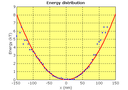
Because the restoring force is proportional to displacement (F = κ·x) and the work done to displace an object from the centre of the trap is given by E=F·x/2, then the potential energy of an object is given by E= κ·x²/2. This results in what is often described as a parabolic “potential well” (see figure).

Potential energy vs. displacement for the record shown previously. The red curve shows the calculated potential energy calculated from the trap stiffness: E = (κ·x²)/2. The blue dots are derived from the probability distribution of the actual data (see figure). The match between the two is close, although the data points become scattered at higher displacements due to the small sample size in the tails of the distribution. No non-linearity is evident.

Contents